Open Access | Peer-reviewed | Research Article
Mehrdad Shahpar*
Director of Ilam Petrochemical Company.
Sharmin Esmaeilpoor
Department of Chemistry, Payame Noor University, P.O. BOX 19395-4697, Tehran, Iran.
Hadi Noorizadeh
Department of Chemistry, Payame Noor University, P.O. BOX 19395-4697, Tehran, Iran.
Published: March 28, 2018 |DOI: 10.5281/zenodo.3372351
Abstract
Environmental hazard is the risk of damage to the environment eg air pollution, water pollution, toxins, and radioactivity. We performed studies upon an extended series of 65 toxic compounds anilines and phenols with chromatographic retention (log k) using quantitative structure–retention relationship (QSRR) methods that imply analysis of correlations and representation of models. A suitable set of molecular descriptors was calculated and the genetic algorithm (GA) was employed to select those descriptors that resulted in the best-fit models. The partial least squares (PLS), kernel partial least squares PLS (KPLS) and Levenberg- Marquardt artificial neural network (L-M ANN) were utilized to construct the linear and nonlinear QSRR models. The proposed methods will be of importance in this research, and could be expected to apply to other similar research fields.
Keywords: Environmental hazard; Ecotoxicity; Phenols; Anilines; Quantitative Stature Retention Relationship; Chemometrics.
| Citation: Mehrdad Shahpar, Sharmin Esmaeilpoor and Hadi Noorizadeh (2018) Modeling of retention behaviors of ecotoxicity of anilines and phenols by chemometrics models. Journal of PeerScientist 1(1): e1000004. doi : 10.5281/zenodo.3372351 |
| Received: August 25, 2017; Accepted March 21, 2018; Published March 28, 2018. |
| Copyright: © 2018 Mehrdad Shahpar et.al. This is an open-access article distributed under the terms of the Creative Commons Attribution License, which permits unrestricted use, distribution, and reproduction in any medium, provided the original author and source are credited. |
| Data Availability: All relevant data are within the paper and its Supporting Information files. |
| Funding: This research received no specific grant from any funding agency in the public, commercial, or not-for-profit sectors. |
| Competing interests: The authors have declared that no competing interests exist. |
| *E-mail: Shahpar2012@gmail.com, hadinoorizadeh@yahoo.com | Phone: + 98-9181432750 |
Introduction
Fathead minnows (Pimephales promelas) are found in every drainage in Minnesota. It is the most common species of minnow in the state. They live in many kinds of lakes and streams, but are especially common in shallow, weedy lakes; bog ponds; low-gradient, turbid (cloudy) streams; and ditches. These habitats often have no predators and low oxygen levels. Fatheads are noted for their ability to withstand low oxygen levels. Fatheads commonly occur with white suckers, bluntnose minnows, common shiners, northern redbelly dace, creek chubs, and young-of-the-year black bullheads. Fathead minnows are considered an opportunist feeder. They eat just about anything that they come across, such as algae, protozoa (like amoeba), plant matter, insects (adults and larvae), rotifers, and copepods. In lakes and deeper streams, fatheads are common prey for crappies, rock bass, perch, walleyes, largemouth bass, and northern pike. They also are eaten by snapping turtles, herons, kingfishers, and terns. Eggs of the fathead are eaten by painted turtles and certain large leeches. Although humans do not eat fatheads, they harvest them as bait [1]. Environmental hazard is a generic term for any situation or state of event which poses a threat to the surrounding natural environment and adversely affects people's health. This term incorporates topics like pollution and natural disasters such as storms and earthquakes. Hazards can be categorized in five types: Chemical, Physical, Mechanical, Biological and Psychosocial. Environmental hazard and risk assessment of chemical substances requires comprehensive information on the exposure, fate and ecotoxicology of the contaminants; however, complete data sets are rarely available. One reason for these deficiencies is that testing capacities are limited, which impedes the thorough experimental investigation of all the existing and new chemicals [2].
To fill at least some of the data gaps, mathematical modeling techniques are used to provide sufficiently accurate substitutes. The models can be used to estimate the parameters related to the fate and effects of chemicals and hence to identify contaminants of special environmental concern and to obtain a ranking of potentially hazardous pollutants. In this way, the priority compounds can then be subjected to detailed testing and the limited resources for experimental investigations can be directed effectively to the chemicals that are most likely to have an environmental impact Attention in mathematical modeling techniques also arises from their application as absolute alternatives to animal experiments, in the interests of time-effectiveness, cost-effectiveness and animal welfare [3].
Alternative methods assist the policy of the “Three Rs” (replacement, reduction and refinement of the use of laboratory animals) and several regulatory organizations have been established to investigate and promote alternative methods. Chemical modeling techniques are based on the premise that the structure of a compound determines all its properties. The study of the type of chemical structure of a foreign substance which will interact to a living system and produce a well-defined biological endpoint is commonly referred to as quantitative structure-retention relationships QSRR [4-5]. The use of QSRR for toxicity estimation of new chemicals or to regulatory toxicological assessment is increasing, especially in aquatic toxicology. Alternatively to QSRR models quantitative retention relationships QRRR, represent other kind of modeling techniques, in which chromatographic retention parameters are used as descriptor and/or predictor variables of a given biological response of chemicals. QSRR models using retention factors (log k) obtained using conventional RP-HPLC, micellar liquid chromatography (MLC) and biopartitioning micellar chromatography (BMC) have been reported [6-10].
The aim of the present study is estimation of ability optimal descriptors calculated with linear regression (the partial least squares (PLS)) and non-linear regressions (the kernel partial least squares (KPLS) and Levenberg- Marquardt artificial neural network (L-M ANN)) in QSRR analysis of logarithm of the retention factor in BMC (log k) for toxicity to Fathead Minnows of anilines and phenols. The stability and predictive power of these models were validated using Leave-Group-Out Cross-Validation (LGO CV) and external test set.
Results and Discussion
Linear model
Results of the GA-PLS model
The best model is selected on the basis of the highest square correlation coefficient leave-group-out cross validation (R2), the least root mean squares error (RMSE) and relative error (RE). These parameters are probably the most popular measure of how well a model fits the data. The best GA-PLS model contains 23 selected descriptors in 11 latent variables space. The R2 and mean RE for training and test sets were (0.788, 0.709) and (15.49, 22.88), respectively. The predicted values of log k are plotted against the experimental values for training and test sets in Figure 1. For this in general, the number of components (latent variables) is less than the number of independent variables in PLS analysis. The PLS model uses higher number of descriptors that allow the model to extract better structural information from descriptors to result in a lower prediction error.
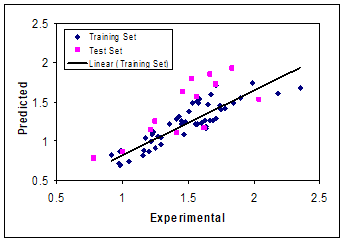
Figure 1: Plots of predicted retention time against the experimental values by GA-PLS model.
Nonlinear model
Results of the GA-KPLS model
In this paper a radial basis kernel function, k(x,y)= exp(||x-y||2/c), was selected as the kernel function with where r is a constant that can be determined by considering the process to be predicted (here r was set to be 1), m is the dimension of the input space and is the variance of the data [11-12]. It means that the value of c depends on the system under the study. The 16 descriptors in 9 latent variables space chosen by GA-KPLS feature selection methods were contained. The R2 and mean RE for training and test sets were (0.811, 0.754) and (13.08, 19.70), respectively. It can be seen from these results that statistical results for GA-KPLS model are superior to GA-PLS method. Figure 2 shows the plot of the GA-KPLS predicted versus experimental values for log k of all of the molecules in the data set.
Results of the L-M ANN model
With the aim of improving the predictive performance of nonlinear QSRR model, L-M ANN modeling was performed. The networks were generated using the sixteen descriptors appearing in the GA-KPLS models as their inputs and log k as their output. For ANN generation, data set was separated into three groups: calibration and prediction (training) and test sets. All molecules were randomly placed in these sets. A three-layer network with a sigmoid transfer function was designed for each ANN. Before training the networks the input and output values were normalized between -1 & 1.
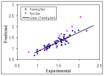
Figure 2: Plots of predicted log k versus the experimental values by GA-KPLS model.
The network was then trained using the training set by the back propagation strategy for optimization of the weights and bias values. The proper number of nodes in the hidden layer was determined by training the network with different number of nodes in the hidden layer. The root-mean-square error (RMSE) value measures how good the outputs are in comparison with the target values. It should be noted that for evaluating the over fitting, the training of the network for the prediction of log k must stop when the RMSE of the prediction set begins to increase while RMSE of calibration set continues to decrease. Therefore, training of the network was stopped when overtraining began. All of the above mentioned steps were carried out using basic back propagation, conjugate gradient and Levenberge-Marquardt weight update functions. It was realized that the RMSE for the training and test sets are minimum when three neurons were selected in the hidden layer. Finally, the number of iterations was optimized with the optimum values for the variables. It was realized that after 18 iterations, the RMSE for prediction set were minimum. The R2 and mean relative error for calibration, prediction and test sets were (0.976, 0.945, 0.887) and (4.14, 5.21, 8.39), respectively. Comparison between these values and other statistical parameter reveals the superiority of the L-M ANN model over other model. The key strength of neural networks, unlike regression analysis, is their ability to flexible mapping of the selected features by manipulating their functional dependence implicitly. The statistical parameters reveal the high predictive ability of L-M ANN model. The whole of these data clearly displays a significant improvement of the QSRR model consequent to nonlinear statistical treatment. Plot of predicted log k versus experimental log k values by L-M ANN for training and test sets are shown in Figure.3a and 3b. Obviously, there is a close agreement between the experimental and predicted log k and the data represent a very low scattering around a straight line with respective slope and intercept close to one and zero. As can be seen in this section, the L-M ANN is more reproducible than other models for modeling the log k of compounds.
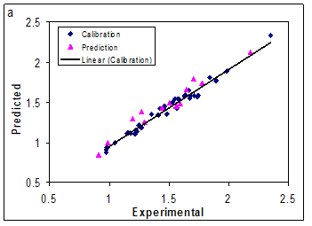
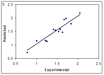
Figure 3: Plot of predicted log k obtained by L-M ANN against the experimental values (a) for training set and (b) test set.
Model validation and statistical parameters
The accuracy of proposed models was illustrated using the evaluation techniques such as leave group out cross-validation (LGO-CV) procedure, validation through an external test set. In addition, chance correlation procedure is a useful method for investigating the accuracy of the resulted model, by which one can make sure if the results were obtained by chance or not. Cross validation is a popular technique used to explore the reliability of statistical models. Based on this technique, a number of modified data sets are created by deleting in each case one or a small group (leave-some-out) of objects. For each data set, an input–output model is developed, based on the utilized modeling technique. Each model is evaluated, by measuring its accuracy in predicting the responses of the remaining data (the ones or group data that have not been utilized in the development of the model). In particular, the LGO-CV procedure was utilized in this study. A QSRR model was then constructed on the basis of this reduced data set and subsequently used to predict the removed data. This procedure was repeated until a complete set of predicted was obtained. The data set should be divided into three new sub-data sets, one for calibration and prediction (training), and the other one for testing. The calibration set was used for model generation. The prediction set was applied deal with over fitting of the network, whereas test set which its molecules have no role in model building was used for the evaluation of the predictive ability of the models for external set [13].
In the other hand by means of training set, the best model is found and then, the prediction power of it is checked by test set, as an external data set. In this work, 60% of the database was used for calibration set, 20% for prediction set and 20% for test set [14], randomly (in each running program, from all 65 components, 39 components are in calibration set, 13 components are in prediction set and 13 components are in test set). The result clearly displays a significant improvement of the QSRR model consequent to non-linear statistical treatment and a substantial independence of model prediction from the structure of the test molecule. In the above analysis, the descriptive power of a given model has been measured by its ability to predict log k of unknown compounds. For the constructed models, two general statistical parameters were selected to evaluate the prediction ability of the model for log k values. For this case, the predicted log k of each sample in the prediction step was compared with the experimental log k. The root mean square error of prediction (RMSE) is a measurement of the average difference between predicted and experimental values, at the prediction stage. The RMSE can be interpreted as the average prediction error, expressed in the same units as the original response values. The RMSEP was obtained using the following formula:![]() The second statistical parameter was the relative error of prediction (RE) that shows the predictive ability of each component, and is calculated as:
The second statistical parameter was the relative error of prediction (RE) that shows the predictive ability of each component, and is calculated as:![]()
![]() Where yi is the experimental log k value of the anilines and phenols in the sample i, represents the predicted log k value in the sample i, is the mean of experimental log k values in the prediction set and n is the total number of samples used in the test set [15].
Where yi is the experimental log k value of the anilines and phenols in the sample i, represents the predicted log k value in the sample i, is the mean of experimental log k values in the prediction set and n is the total number of samples used in the test set [15].
Conclusion
The GA-PLS, GA-KPLS and L-M ANN models was applied for the prediction of the log k values of ecotoxicity of anilines and phenols. High correlation coefficients and low prediction errors confirmed the good predictability of models. All methods seemed to be useful, although a comparison between these methods revealed the slight superiority of the L-M ANN over other models. Application of the developed model to a testing set of 13 compounds demonstrates that the new model is reliable with good predictive accuracy and simple formulation. The QSRR procedure allowed us to achieve a precise and relatively fast method for determination of log k of different series of these compounds to predict with sufficient accuracy the log k of new substituted compounds.
Materials and Methods
Computer hardware and software
A Pentium IV personal computer (CPU at 3.06 GHz) with the Windows XP operating system was used. The structures of the compounds were drawn with HyperChem version 7.0. All molecules were pre-optimized using molecular mechanics AM1 method in the HyperChem program. The output files exported from Dragon for generating descriptors which was developed by Todeschini et al [16]. The GA-PLS, GA-KPLS, L-M ANN, cross validation and other calculations were performed in MATLAB (Version 7.0, Math works, Inc).
Data set
The 65 phenols and anilines for which experimental chromatographic retention (log k) values to Fathead minnows were available [17] [Ren et al., 2003] were used. The name of studied compounds and their experimental log k values for training and test sets are shown in Table 1 and Table 2. These data were obtained by bio partitioning micellar chromatography. An Agilent 1100 chromatograph with a quaternary pump and an UV–vis detector (variable wavelength detector) was employed.
Table 1: The compounds and log retention factor for calibration and prediction sets:
| S.No | Compounds | Log K |
| Calibration set | ||
| 1. | 2,6-Dimethoxiphenol | 0.976 |
| 2. | 2,5-Dinitrophenol | 0.977 |
| 3. | 4,6-Dinitro-2-methylphenol | 0.979 |
| 4. | 3-Hydroxyphenol | 1.05 |
| 5. | 2,3,6-Trichlorophenol | 1.152 |
| 6. | 4-Methoxyphenol | 1.16 |
| 7. | 2,3,4,6-Tetrachlorophenol | 1.176 |
| 8. | 4-Nitrophenol | 1.218 |
| 9. | Pentachlorophenol | 1.224 |
| 10. | 4-Methylaniline | 1.226 |
| 11. | 2,4,6-Trichlorophenol | 1.227 |
| 12. | Phenol | 1.246 |
| 13. | 3-Methoxyphenol | 1.268 |
| 14. | 2,6-Dichlorophenol | 1.292 |
| 15. | N-Methylaniline | 1.352 |
| 16. | 4-Mehtylphenol | 1.41 |
| 17. | 3-Nitrophenol | 1.426 |
| 18. | 2-Chlorophenol | 1.45 |
| 19. | 2-Methylphenol | 1.465 |
| 20. | 2,4-Dinitroaniline | 1.481 |
| 21. | 4-Chlorophenol | 1.529 |
| 22. | 4-Ethylphenol | 1.55 |
| 23. | 2,3,5-Trichlorophenol | 1.564 |
| 24. | 3,4-Dichloroaniline | 1.566 |
| 25. | 2-Chloro-4-methylaniline | 1.575 |
| 26. | 2,6-Dichloro-4-aniline | 1.583 |
| 27. | 2,4,6-Trimethylphenol | 1.627 |
| 28. | 2,4-Dichlorophenol | 1.632 |
| 29. | 2,4,5-Trichlorophenol | 1.633 |
| 30. | 2,3,4-Trichloroaniline | 1.668 |
| 31. | Pentafluoroaniline | 1.67 |
| 32. | 4-Phenoxiphenol | 1.681 |
| 33. | 4-Butylaniline | 1.71 |
| 34. | 3,4,5-Trichlorophenol | 1.741 |
| 35. | 4-Tert-butylphenol | 1.746 |
| 36. | 4-Tert-pentylphenol | 1.839 |
| 37. | 2,6-Diisopropylaniline | 1.897 |
| 38. | 2,6-Diisopropylphenol | 1.988 |
| 39. | 2,6-Di(tert)butil-4-methylphenol | 2.351 |
| Prediction Set | ||
| 40. | 2,4-Dinitrophenol | 0.913 |
| 41. | Aniline | 0.986 |
| 42. | 2,3,5,6-Tetrachlorophenol | 1.199 |
| 43. | 4-Nitroaniline | 1.266 |
| 44. | 2,4,6-Triiodophenol | 1.293 |
| 45. | 4-Ethylaniline | 1.445 |
| 46. | 2-Chloro-4-nitroaniline | 1.501 |
| 47. | 2,3,4,5-Tetrachlorophenol | 1.565 |
| 48. | 4-Chloro-3-methylphenol | 1.596 |
| 49. | N,N-Dimethylaniline | 1.644 |
| 50. | 2-Phenylphenol | 1.706 |
| 51. | 4-Hexyloxyaniline | 1.775 |
| 52. | Nonylphenol | 2.183 |
It is equipped with a column thermostat with 9L extra-column volume for preheating mobile phase prior to the column and an auto sampler with a 20 L loop. All the assays were carried out at 25 ◦C. Data acquisition and processing were performed by means of an HP Vectra XM computer (Amsterdam, The Netherlands) equipped with HP-Chemstation software (A.07.01 [682] ©HP 1999). Two Kromasil C18 columns (5 m, 150mm × 4.6mm i.d.; Scharlab S.L., Barcelona, Spain) and (5 m, 50mm × 4.6mm i.d.; Scharlab) were used. The mobile phase flow rate was 1.0 or 1.5mLmin−1 for the 150 mm and 50 mm column length, respectively. The detection was performed in UV at 254 nm for acetanilide, antipyrine and propiophenone (reference compounds), and 240 nm for phenols and anilines.
Table 2: The data set and log k for test set:
| S.No | Compounds | Log K |
| 1. | 2,6-Dinitrophenol | 0.779 |
| 2. | 2-Nitrophenol | 0.999 |
| 3. | 2,4,6-Tribromophenol | 1.216 |
| 4. | Pentabromophenol | 1.249 |
| 5. | 4-Chloroaniline | 1.408 |
| 6. | 2-Chloroaniline | 1.459 |
| 7. | 4-Ethoxy-2-nitroaniline | 1.527 |
| 8. | 2,4-Dimethylphenol | 1.567 |
| 9. | 2,3,6-Trimethylphenol | 1.623 |
| 10. | 4-Propylphenol | 1.666 |
| 11. | 3,5-Dichlorophenol | 1.709 |
| 12. | 2,3,5,6-Tetrachloroaniline | 1.833 |
| 13. | 4-Octylaniline | 2.042 |
Determination of molecular descriptors
Molecular descriptors are defined as numerical characteristics associated with chemical structures. The molecular descriptor is the final result of a logic and mathematical procedure which transforms chemical information encoded within a symbolic representation of a molecule into a useful number applied to correlate physical properties. The Dragon software was used to calculate the descriptors in this research and a total of molecular descriptors, from 18 different types of theoretical descriptors, were calculated for each molecule. Since the values of many descriptors are related to the bonds length and bonds angles etc., the chemical structure of every molecule must be optimized before calculating its molecular descriptors. For this reason, the chemical structure of the 65 studied molecules were drawn with Hyperchem software and saved with the HIN extension. To optimize the geometry of these molecules, the AM1 geometrical optimization was applied. After optimizing the chemical structures of all compounds, the molecular descriptors were calculated using Dragon. A wide variety of descriptors have been reported in the literature, having been used in QSRR analysis.
Genetic algorithm for descriptor selection
In QSRR studies, after calculating the molecular descriptors from optimized chemical structures of all the components available in the data set, the problem is to find an equation that can predict the desired property with the least number of variables as well as highest accuracy. In other words, the problem is to find a subset of variables (most statistically effective molecular descriptors for the log k) from all the available variables (all molecular descriptors) that can predict log k with the minimum error in comparison to the experimental data. A generally accepted method for this problem is the genetic algorithm based linear and non linear regressions (GA-PLS and GA-KPLS). In these methods, the genetic algorithm is applied for the selection of the best subset of variables with respect to an objective function.
GA is a stochastic optimization method that has been inspired by evolutionary principles. The distinctive aspect of GA is that it investigates many possible solutions simultaneously, each of which explores different regions in parameter space. GA has been applied as an optimization technique in several scientific fields [18-19]. In GA for variable selection, the chromosome and its fitness in the species represent a set of variables and predictivity of the derived QSRR model, respectively. GA consists of three basic steps: (1) An initial population of chromosomes is created. The number of the population is dependent on the dimensions of application problems. A binary bit string represents each chromosome. Bit “1” denotes a selection of the corresponding variable, and bit “0” denotes a non selection. The values of a binary bit are determined in a random way (probability of initial variable selection). (2) A fitness of each chromosome in the population is evaluated by predictivity of the QSRR model derived from the binary bit string. (3) The population of chromosomes in the next generation is reproduced. The third step can be divided into three operations: selection, crossover, and mutation. The application probability of these operators was varied linearly with a generation renewal. For a typical run, the evolution of the generation was stopped, when 90% of the generations had taken the same fitness. In this paper, size of the population is 30 chromosomes, the probability of initial variable selection is 5:V (V is the number of independent variables), crossover is multi Point, the probability of crossover is 0.5, mutation is multi Point, the probability of mutation is 0.01 and the number of evolution generations is 1000. For GA-PLS and GA-KPLS programs, 3000 runs were performed.
Data pre-processing
Each set of the calculated descriptors was collected in a separate data matrix Di with a dimension of (m×n), where m and n are being the number of molecules and the number of descriptors, respectively. Grouping of descriptors was based on the classification achieved by Dragon software. In each group, the calculated descriptors were searched for constant or near constant values for all molecules and those detected were removed. Before applying the analysis methods, and due to the quality of data, a previous treatment of the data is required. Scaling and centering is one of the pre-processing methods we need before performing the regression methods combined with FE. The results of projection methods depend on the normalization of the data. Descriptors with small absolute values have a small contribution to overall variances; this biases towards other descriptors with higher values. With appropriate scaling, equal weights are assigned to each descriptor, so that the important variables in the model can be focused. In order to give all variables the same importance, they are standardized to unit variance and zero mean (autoscaling).
Nonlinear model
Artificial neural network
A three-layer back propagation artificial neural network ANN with a sigmoid transfer function was used in the investigation of feature sets. The descriptors from the calibration set were used for the model generation whereas the descriptors from the prediction set were used to stop the overtraining of network. And the descriptors from the test set were used to verify the predictivity of the model. Before training the networks, the input and output values were normalized with auto-scaling of all data [20-21]. The goal of training the network is to minimize the output errors by changing the weights between the layers.![]() In this, is the change in the weight factor for each network node, α is the momentum factor, and F is a weight update function, which indicates how weights are changed during the learning process. The weights of hidden layer were optimized using the Levenberg-Marquardt algorithm, a second derivative optimization method [22].
In this, is the change in the weight factor for each network node, α is the momentum factor, and F is a weight update function, which indicates how weights are changed during the learning process. The weights of hidden layer were optimized using the Levenberg-Marquardt algorithm, a second derivative optimization method [22].
Levenberg-Marquardt Algorithm
In Levenberg-Marquardt algorithm, the update function, Fn, is calculated using equations.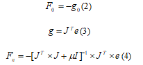 Where g is gradient and J is the Jacobian matrix that contains first derivatives of the network errors with respect to the weights, and e is a vector of network errors. The parameter µ is multiplied by some factor (λ) whenever a step would result in an increased e and when a step reduces e, µ is divided by λ [23].
Author Contributions
MS, SE & HN has conceived, executed and analyzed the data for the presented idea. All authors discussed the results and contributed to the final manuscript.
References
- Sowers, Anthony D., et al. "Developmental effects of a municipal wastewater effluent on two generations of the fathead minnow, Pimephales promelas." Aquatic toxicology95.3 (2009): 173-181.
- Aruoja, Villem, et al. "Effect of substituents on the ecotoxicity of anilines and phenols." Toxicology Letters 189 (2009): S192.
- Al-Awadhi, J. M., and A. A. Al-Awadhi. "Modeling the aeolian sand transport for the desert of Kuwait: constraints by field observations." journal of arid Environments 73.11 (2009): 987-995.
- Duchowicz, Pablo R., et al. "Quantitative structure–property relationship analyses of aminograms in food: Hard cheeses." Chemometrics and Intelligent Laboratory Systems 107.2 (2011): 384-390.
- Goodarzi, Mohammad, Tao Chen, and Matheus P. Freitas. "QSPR predictions of heat of fusion of organic compounds using Bayesian regularized artificial neural networks." Chemometrics and Intelligent Laboratory Systems 104.2 (2010): 260-264.
- Liu, Tao, Ian A. Nicholls, and Tomas Öberg. "Comparison of theoretical and experimental models for characterizing solvent properties using reversed phase liquid chromatography." Analytica chimica acta 702.1 (2011): 37-44.
- Kaliszan, Roman, et al. "Thermodynamic vs. extrathermodynamic modeling of chromatographic retention." Journal of Chromatography A 1218.31 (2011): 5120-5130.
- Flieger, J. "Application of perfluorinated acids as ion-pairing reagents for reversed-phase chromatography and retention-hydrophobicity relationships studies of selected β-blockers." Journal of Chromatography A 1217.4 (2010): 540-549.
- Buciński, Adam, et al. "Artificial neural networks analysis used to evaluate the molecular interactions between selected drugs and human α1-acid glycoprotein." Journal of pharmaceutical and biomedical analysis 50.4 (2009): 591-596.
- Lämmerhofer, Michael. "Chiral recognition by enantioselective liquid chromatography: mechanisms and modern chiral stationary phases." Journal of Chromatography A 1217.6 (2010): 814-856.
- Jia, Run-Da, et al. "Kernel partial robust M-regression as a flexible robust nonlinear modeling technique." Chemometrics and Intelligent Laboratory Systems 100.2 (2010): 91-98.
- Jalali-Heravi, Mehdi, and Anahita Kyani. "Application of genetic algorithm-kernel partial least square as a novel nonlinear feature selection method: activity of carbonic anhydrase II inhibitors." European journal of medicinal chemistry 42.5 (2007): 649-659.
- Noorizadeh, Hadi, and Mehrab Noorizadeh. "QSRR-based estimation of the retention time of opiate and sedative drugs by comprehensive two-dimensional gas chromatography." Medicinal Chemistry Research 21.8 (2012): 1997-2005.
- Chen, Hai-Feng. "Quantitative predictions of gas chromatography retention indexes with support vector machines, radial basis neural networks and multiple linear regression." Analytica chimica acta 609.1 (2008): 24-36.
- Deeb, Omar. "Correlation ranking and stepwise regression procedures in principal components artificial neural networks modeling with application to predict toxic activity and human serum albumin binding affinity." Chemometrics and Intelligent Laboratory Systems 104.2 (2010): 181-194.
- Todeschini, R., et al. "DRAGON-Software for the calculation of molecular descriptors." Web version 3 (2004).
- Ren, Shijin, Paul D. Frymier, and T. Wayne Schultz. "An exploratory study of the use of multivariate techniques to determine mechanisms of toxic action." Ecotoxicology and environmental safety 55.1 (2003): 86-97.
- Sarıpınar, Emin, et al. "Pharmacophore identification and bioactivity prediction for triaminotriazine derivatives by electron conformational-genetic algorithm QSAR method." European journal of medicinal chemistry 45.9 (2010): 4157-4168.
- Sagrado, Salvador, and Mark TD Cronin. "Application of the modelling power approach to variable subset selection for GA-PLS QSAR models." Analytica chimica acta 609.2 (2008): 169-174.
- Hernández-Caraballo, Edwin A., et al. "Evaluation of chemometric techniques and artificial neural networks for cancer screening using Cu, Fe, Se and Zn concentrations in blood serum." Analytica Chimica Acta 533.2 (2005): 161-168.
- Gupta, Vinod Kumar, et al. "Prediction of capillary gas chromatographic retention times of fatty acid methyl esters in human blood using MLR, PLS and back-propagation artificial neural networks." Talanta 83.3 (2011): 1014-1022.
- Bolanča, Tomislav, et al. "Development of an inorganic cations retention model in ion chromatography by means of artificial neural networks with different two-phase training algorithms." Journal of Chromatography A 1085.1 (2005): 74-85.
- Chamjangali, M. Arab, M. Beglari, and G. Bagherian. "Prediction of cytotoxicity data (CC50) of anti-HIV 5-pheny-l-phenylamino-1H-imidazole derivatives by artificial neural network trained with Levenberg–Marquardt algorithm." Journal of Molecular Graphics and Modelling 26.1 (2007): 360-367.